It denotes M – 1 auxiliary beams, output of matrix prefilter B, and is given by
![]()
(6.6)
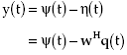
It follows from the Figure 9 that the output of the main beam ψ(t) is given by
| (6.3) | |
| where the L-dimensional vector V is defined as | |
| (6.4) | |
| Let an M – 1 dimensional vector q(t) be defined as | |
| (6.5) | |
It denotes M – 1 auxiliary beams, output of matrix prefilter B, and is given by
|
(6.6) |
(6.7) |
 |
(6.8) |
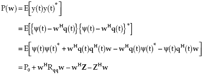 |
(6.9) |
| where P0 is the mean power of the main beam given by | |
(6.10) |
|
| Rqq is the correlation matrix of auxiliary beams defined as | |
(6.11) |
| (6.12) | |
| A substitution for q(t) and ψ(t) in (6.11) and (6.12) yields | |
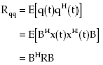 |
(6.13) |
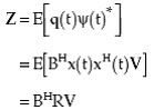 |
(6.14) |
| Substituting for P0, Rqq and Z in (6.9), the expression for P(w) becomes | |
| (6.15) |
(6.16) |
|
| Substituting (6.15) in (6.16) yields | |
(6.17) |
(6.18) |
(6.19) |
| (6.20) | |
| Since | |
| (6.21) | |
| and | |
| (6.22) | |
| it follows from (6.20) that | |
| (6.23) |
| (6.24) |
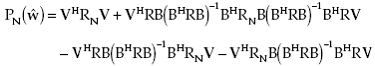
| (6.25) |
| (6.26) |
 |
(6.27) |
| (6.28) |
These expressions cannot be simplified further without considering specific cases. Later , a special case of beam space processor is considered where only one auxiliary beam is considered in the presence of one interference source to understand the behavior of beam space processors. The results are then compared with an element space processor. In the next section, a beam space processor referred to as the generalized side-lobe canceler (GSC) is considered. The main difference between the general beam space processor considered in this section and the GSC is that the GSC uses presteering delays.
In the next page Generalized Side-Lobe Canceler is discussed.
Back To Contents.