Untitled Document

In contrast to the element space processing, where signals derived from each element are weighted and summed to produce the array output, the beam space processing is a two-stage scheme where the first stage takes the array signals as input and produces a set of multiple outputs, which are then weighted and combined to produce the array output. These multiple outputs may be thought of as the output of multiple beams. The processing done at the first stage is by fixed weighting of the array signals and amounts to produce multiple beams steered in different directions. The weighted sum of these beams is produced to obtain the array output and the weights applied to different beam outputs are then optimized to meet a specific optimization criterion.

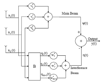
In general, for an L-element array, a beam space processor consists of a main beam steered in the signal direction and a set of not more than L – 1 secondary beams. The weighted output of the secondary beams is subtracted from the main beam. The weights are adjusted to produce an estimate of the interference present in the main beam. The subtraction process then removes this interference. The secondary beams, also known as auxiliary beams, are designed such that they do not contain the desired signal from the look direction, to avoid signal cancelation in the subtraction process. A general structure of such a processor is shown in Figure 9. Beam space processors have been studied under many different names including the Optimum beam space processor,Howells–Applebaum array, generalized side-lobe canceler (GSC), partitioned processor, partially adaptive arrays, post-beamformer interference canceler,adaptive-adaptive arrays, and multiple-beam antennas.

The pattern of the main beam is normally referred to as the quiescent pattern and is chosen such that it has a desired shape. For a linear array of equispaced elements with equal weighting, the quiescent pattern has the shape of sin Lx/sin x with L being the number of elements in the array, whereas for Tschebysheff weighting (the weighting dependent on Tschebysheff polynomial coefficients), the pattern has equal side-lobe levels. The beam pattern of the main beam may be adjusted by applying various forms of constraints on the weights and using various pattern synthesis techniques.

There are many schemes to generate the outputs of auxiliary beams such that no signal from the look direction is contained in them, that is, these beams have nulls in the look direction. In its simplest form, it can be achieved by subtracting the array signals from presteered adjacent pairs. It relies on the fact that the component of the array signals induced from a source in the look direction is identical after the presteering, and this gets canceled in the subtraction process from the adjacent pairs. The process can be generalized to produce M – 1 beams from an L-element array signal x(t) using a matrix B such that

where M – 1 dimensional vector q(t) denotes the outputs of M – 1 beams and the matrix B, referred to as the blocking matrix or the matrix prefilter, has the property that its M – 1 columns are linearly independent and the sum of elements of each column equals zero, implying that M – 1 beams are independent and have nulls in the look direction. For an array that is not presteered, the matrix needs to satisfy

where S0 is the steering vector associated with the look direction and 0 denotes a vector of zeros.

It is assumed in the above discussion that M ≤ L, implying that the number of beams are less than or equal to the number of elements in the array. When the number of beams is equal to the number of elements in the array, the processing in the beam space has not reduced the degree of freedom of the array, that is, its null-forming capability has not been reduced. In this sense, these arrays are fully adaptive and have the same capabilities as that of the array using element space processing. In fact, in the absence of errors, both processing schemes produce identical results. On the other hand, when the number of beams is less than the number of elements, the arrays are referred to as partially adaptive. The null steering capabilities of these arrays have been reduced to equal the number of auxiliary beams. However, the MSE for these arrays is also high compared to fully adaptive arrays.

These arrays are useful in situations where the number of interferences are much less than the number of elements and offer computational advantage over element space processing, as you only need to adjust M – 1 weights compared to L weights for the element space case with M < L. Moreover, beam space processing requires less computation than the element space case to calculate the weights in general as it solves an unconstrained optimization compared to the constrained optimization problem solved in the latter case. It should be noted that for the element space processing case, constraints on the weights are imposed to prevent distortion of the signal arriving from the look direction and tomake the array more robust against errors. For the beam space case, constraints are transferred to the main beam, leaving the adjustable weights free from constraints.

Auxiliary beamforming techniques other than the use of a blocking matrix described above include formation of M – 1 orthogonal beams and formation of beams in the direction of interference, if known. The beams are referred to as orthogonal beams to imply that the weight vectors used to form beams are orthogonal, that is, their dot product is equal to zero. The eigenvectors of the array correlation matrix taken as weights to generate auxiliary beams fall into this category. In situations where directions of arrival of interference are known, the formation of beams pointed in these directions may lead to more efficient interference cancelation.

Auxiliary beam outputs are weighted and summed, and the result is subtracted from the main beam output to cancel the unwanted interference present in the main beam. The weights are adjusted to cancel the maximum possible interference. This is normally done by minimizing the total mean output power after subtraction by solving the unconstrained optimization problem and leads to maximization of the output SNR in the absence of the desired signal in auxiliary channels. The presence of the signal in these channels causes signal cancelation from the main beam along with interference cancelation.