Home > Spectrum Managment > Spectrum Sensing > Transmitter Detection > Energy Detection

Power-based sensing can be performed in both time domain and frequency domain. To measure the signal power in a particular frequency region in time domain, a bandpass filter is applied to the target signal and the power of the signal samples (after the filter) is then measured.
To measure the signal power in frequency domain, the time-domain signal is transformed to frequency domain using FFT and the combined signal power over all frequency bins in the target frequency region is then measured. For either case, we consider the received signal of the form

where x(n) is the target signal; z(n) is the white Gaussian noise; and n the sample index in the case of time-domain sensing, or FFT symbol index in the case of frequency-domain sensing. For simplicity of derivation, we will assume the signal sample x(n)s are independent. Correlation among signal sample x(n)s, e.g. due to multipath channel memory effect, will only improve the sensing performance. Since the noise sample z(n)s are also independent, the received sample y(n)s are independent. Consider using the following signal power sum as the power sensing metric:

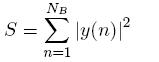
where NB is the summing buffer size. Note that |y(n)|2 is a sequence of independent and identically distributed (IID) random variables with mean and variance

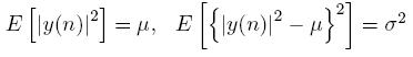
When NB is large, using central limit theorem, the sensing metric S can be approximated as a Gaussian random variable with mean and variance

When there is no signal present, i.e. x(n) = 0, the sensing metric is:

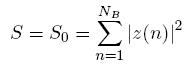
When there is signal present, the sensing metric is:

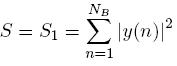
Figure 1 shows the distributions of S0 and S1, which are Gaussians.

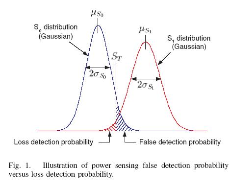
The signal presence is determined by comparing the measured sensing metric S against certain sensing threshold ST . Referring to the figure, false detection probability (PFD) is the probability that S > ST when there is no signal present and the loss detection probability (PLD) is the probability that S < ST when there is signal present. The tradeoff between PFD and PLD leads to the optimal sensing threshold ST, when the PFD is equal to the PLD. We define the sensing error floor (SEF) as the PFD (or PLD) at the optimal threshold. Since both PFD and PLD are Gaussian tail integrations that can be expressed in terms of the Q function:

the optimal sensing threshold ST is found by equating the arguments of the above Q functions:

Thus we obtain the sensing error floor:

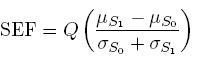
It can be shown, after some mathematical steps, the sensing error floor can be expressed in terms of the signal-to-noise ratio and summing buffer size as:

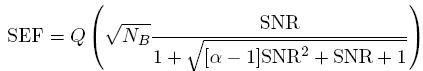
Here

is the nominal symbol SNR and

is an intrinsic parameter of the signal x(n) that relates its randomness. For example, for complex Gaussian signal, α is 2. For constant-amplitude signals, e.g. BPSK, QPSK, and 8-PSK, α is 1. For other types of signals, α is between 1 and 2.

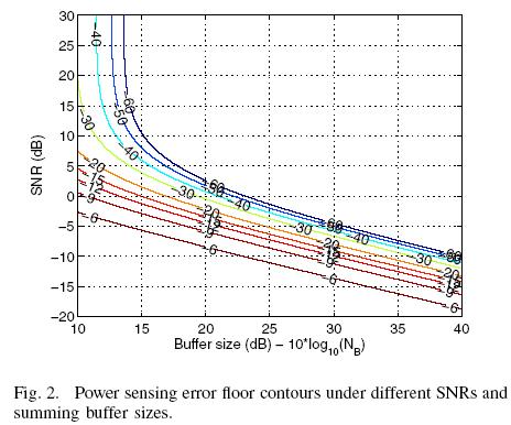
Figure 2 shows the sensing error floor contours at different SNRs and summing buffer sizes, with α = 2 (Gaussian signal). Note that the error floor is expressed in dB units, e.g. -20 dB corresponding to 0.01.